10. Area and Average Value

d. Average Value and Mean Value Theorem

Recall: The average value of a function \(f(x)\) on an interval \([a,b]\) is: \[ f_\text{ave}=\dfrac{1}{b-a}\int_a^b f(x)\,dx \]

2. Average Value and Area

Notice that the formula for the average value of a function can be rewritten as \[ \int_a^b f(x)\,dx=(b-a)f_\text{ave} \]

When \(f(x)\) is positive, the integral on the left is just the area under \(y=f(x)\) and the product on the right is the area of a rectangle with width \(b-a\) and height \(f_\text{ave}\). Thus we conclude:

The average value \(f_\text{ave}\) of a positive function \(f(x)\) is the height of a rectangle of width \(b-a\) whose area is the same as the area under \(y=f(x)\) over the interval \([a,b]\).

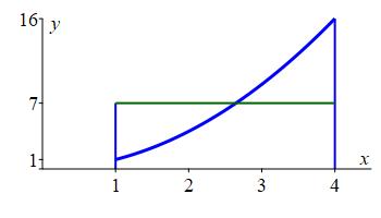
Plot the function \(y=x^2\) and its average value on the interval \([1,4]\) and note the relation between the areas below the curves.

The average value was found in a previous example to be \(f_\text{ave}=7\). Notice in the graph to the right, that the area under the blue curve and the area under the green line are both \(21\).
Equivalently, the part of the area under the blue curve above the green line (shown in orange). balances the part below the green line above the blue curve (shown in cyan).

Now you try it:

Plot the function \(y=(x-2)^2\) and its average value on the interval \([1,3]\) and note the relation between the areas below the curves.

Here is the graph:

The area below the blue curve is equal to the area below the green line.
Equivalently, the part of the area under the blue curve above the green line (shown in orange). balances the part below the green line above the blue curve (shown in cyan).

The average value was found, in a previous exercise, to be \(f_\text{ave}=\dfrac{1}{3}\). Thus the graph is:

Notice the area below the blue curve is equal to the area below the green line.
Equivalently, the part of the area under the blue curve above the green line (shown in orange). balances the part below the green line above the blue curve (shown in cyan).

And now an application:

A fish tank which is \(40\) cm long and \(25\) cm deep has a water wave whose shape (at one instant of time) is given by \[ y(x)=\dfrac{1}{1000}x^3-\dfrac{11}{200}x^2+\dfrac{4}{5}x+16 \] as shown in the figure. If the water is allowed to come to equilibrium (so the water level is constant), what will be the depth of the water? Assume the water is incompressible.

The equilibrium depth will be the average depth \(y_\text{ave}=\dfrac{56}{3}\approx 18.7\) cm.

Since the water is incompressible, the volume of the water is the same before and after it reaches equilibrium. So the area under the curve will equal the area of the final rectangle whose height is the average of the height of the curve. \[\begin{aligned} y_\text{ave} &=\dfrac{1}{40}\int_0^{40} \left(\dfrac{1}{1000}x^3-\dfrac{11}{200}x^2+\dfrac{4}{5}x+16\right)\,dx \\ &=\dfrac{1}{40} \left[\dfrac{x^4}{4000}-\dfrac{11x^3}{600}+\dfrac{2x^2}{5}+16x\right]_0^{40} \\ &=\dfrac{1}{40} \left(\dfrac{40^4}{4000}-\dfrac{11\cdot40^3}{600}+\dfrac{2\cdot40^2}{5}+16\cdot40\right) \\ &=\dfrac{56}{3}\approx18.7\text{cm} \end{aligned}\]

You can practice estimating and computing Average Values by using the Tutorial at the end of this chapter. In the first half of the Tutorial, you get to estimate the average value using areas, while in the second half you compute it exactly.

You can also practice estimating and computing Average Values by using the following Maplet (requires Maple on the computer where this is executed):

Average Value of a Function Rate It

In the first half of the Maplet, you get to estimate the average value using areas, while in the second half you compute it exactly.

10. Area and Average Value

d. Average Value and Mean Value Theorem

2. Average Value and Area

Heading